Neural DNA (NDNA)
A compact genome for growing neural network architecture
First, Some Context
When people talk about AI, they are usually talking about AI models: systems like ChatGPT, image generators, or voice assistants. These models are built on something called a neural network, a structure loosely inspired by how the brain processes information.
A neural network is made up of layers of "neurons" connected to each other. When you train an AI, two things happen:
- Architecture: Someone decides the structure of the network. How many layers? How many neurons? Which neurons connect to which? This is usually done by hand, by engineers making educated guesses.
- Learning: The network is shown thousands or millions of examples (images, text, data) and it adjusts the strength of its connections to get better at its task. This is the "training" part.
NDNA is about step 1. It is not about what the AI learns, but about how the AI's brain is wired in the first place.
The Problem
Today, most neural networks use a brute-force approach to architecture: connect everything to everything. Every neuron in one layer connects to every neuron in the next. This is called a "dense" or "fully-connected" network. It works, but it is wasteful. Most of those connections end up not contributing much, and the ones that do matter get buried among thousands of useless ones.
This is like building a city where every house has a direct road to every other house. It would technically work, but it would be absurdly expensive, most roads would never be used, and the useful routes would be lost in the noise.
The human brain does not work this way. During development, neurons grow their connections selectively. An axon extends, finds compatible targets, and forms a synapse only where it is useful. Maintaining a synapse costs energy (metabolic cost), so the brain is forced to be selective. The result is a brain with roughly 100 trillion synapses, but that is actually a tiny fraction of all possible connections. The brain is sparse by design.
NDNA asks: what if AI networks could grow their own wiring the same way?
What NDNA Does
Instead of an engineer hand-designing the network structure, NDNA introduces a tiny "genome" (fewer than 400 numbers) that learns which connections should exist. The genome does not store the connections themselves. It stores the rules for growing them, just like biological DNA does not store your body directly but stores the instructions for building it.
During training, the genome evaluates every possible connection in the network and decides: should this wire exist, or not? A metabolic cost penalty punishes the genome for growing too many connections, forcing it to be selective. Only connections that actually help the network perform better survive.
The result: genomes with 226 to 374 parameters control networks with up to 2.2 million possible connections. The highest compression we measured is 8,384:1, where 258 genome parameters control 2.16 million transformer connections. Even the "smallest" experiment compresses at 770:1. These ratios are likely even higher on larger networks. A tiny blueprint grows an entire brain.
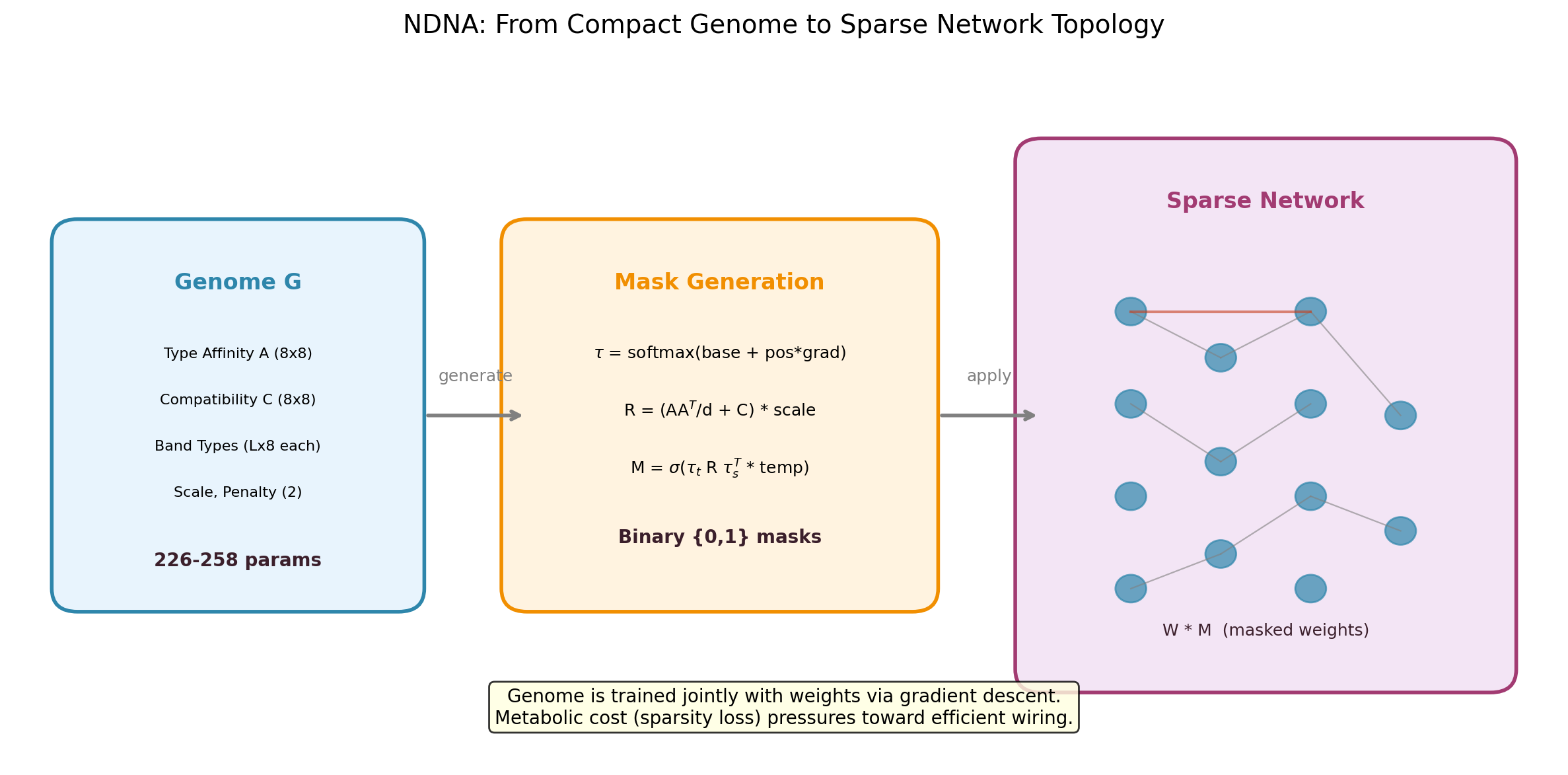
The NDNA pipeline. A small genome encodes "cell types" and a compatibility matrix. During growth, it checks every potential connection: are the source and target neurons compatible? If yes, the connection gets made. If not, it stays disconnected. The resulting sparse network trains alongside the genome.
Where NDNA Fits in the AI Pipeline
To put this in perspective, here is where different parts of AI research focus:
- Data: Collecting and cleaning the examples the AI learns from (images, text, etc.)
- Architecture (this is where NDNA lives): Designing the structure and wiring of the network itself
- Training: The process of adjusting connection strengths so the network gets better at its task
- Inference: Using the trained network to make predictions on new data
Most AI research focuses on training techniques, data quality, or scaling up. NDNA focuses on the architecture question: before you even start training, what should the network's wiring look like? Today this is done by hand (or by expensive search algorithms). NDNA automates it with a biological growth process.
How It Works (Step by Step)
-
Genome: A small set of numbers that represents "cell types" (8 types, 8 dimensions each) and a compatibility matrix. Think of it as DNA: a compact blueprint that contains the rules for building something much larger.
-
Growth: For each potential connection in the network, the genome looks at what type the source neuron is and what type the target neuron is. It runs them through the compatibility matrix and outputs a probability. High compatibility = connection gets made. Low compatibility = no connection.
-
Decision: The probabilities are converted into hard yes/no decisions. This produces a "mask", a map of which connections exist and which do not.
-
Metabolic cost: A penalty that punishes the genome for growing too many connections. Just like a biological brain cannot afford to maintain infinite synapses, the genome is forced to keep only the connections that earn their place.
-
Default disconnected: Everything starts disconnected. The genome must actively grow each connection. This is the opposite of the traditional approach (start fully connected, then prune). Growing from nothing means every connection has to justify its existence.
The genome and the network train together. The genome learns what structure to grow. The network weights learn what to do within that structure. Both improve simultaneously.
Why This Matters
Compression. A few hundred numbers encode the wiring plan for millions of connections. This is not incremental. It is a fundamentally different way to think about network design.
Efficiency. The grown networks are sparse (mostly disconnected) but structured. They use a fraction of the connections a dense network would, while performing just as well or better.
Transferability. A genome trained on one task can grow useful wiring for a completely different task, without retraining. This suggests the genome learns something fundamental about how information should flow, not just task-specific tricks.
Biology-inspired. NDNA borrows principles from neuroscience (selective growth, metabolic cost, cell types) and applies them to artificial networks. This is not just metaphor; these principles are what make the approach work.
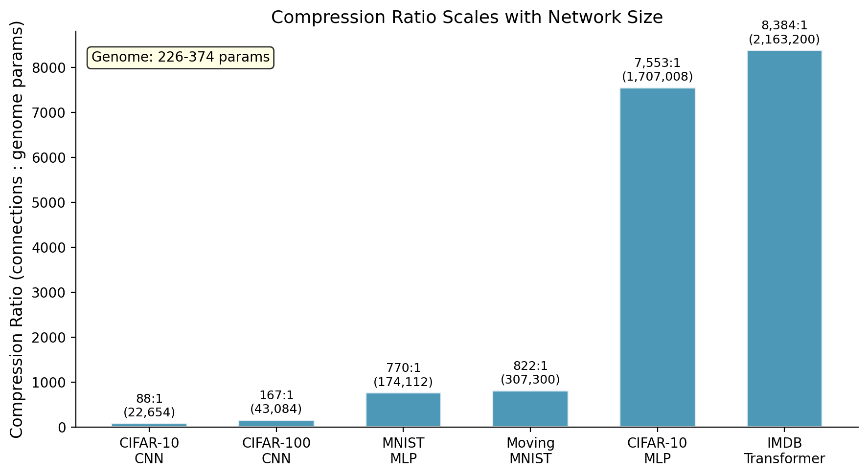
How much compression each genome achieves. The transformer hits 8,384:1 (258 parameters controlling 2.16 million connections). The CIFAR-10 MLP reaches 7,553:1 (226 parameters, 1.7 million connections). The video transformer achieves 821:1 (374 parameters, 307K connections). The CNN is lower because convolutional layers have fewer total connections to begin with.
Key Results
We tested NDNA across six experiments, covering four different network architectures (MLP, CNN, Transformer, Video Transformer) and five different datasets.
| Experiment | Genome | Random Sparse | Dense Baseline | Genome vs Random |
|---|---|---|---|---|
| MNIST (MLP) | 97.54% | 97.09% | 98.33% | +0.45% |
| CIFAR-10 (MLP) | 57.14% | 51.68% | 54.32% | +5.46% |
| CIFAR-10 (CNN) | 88.93% | 85.78% | 89.80% | +3.15% |
| CIFAR-100 (Transfer) | 60.92% | 53.91% | 67.16% | +7.01% |
| IMDB (Transformer) | 85.05% | 84.66% | 84.57% | +0.39% |
| Moving MNIST (Video)* | 62.23 | 79.44 | 62.15 | +21.7% |
*Moving MNIST uses MSE (lower is better). The +21.7% is relative improvement: random sparse MSE is 21.7% worse than genome MSE.
How to read this table:
- Genome: NDNA's result. The network whose wiring was grown by the genome.
- Random Sparse: A network with the same number of connections as the genome network, but wired randomly. This is the control: does learned wiring actually matter, or would any sparse wiring do?
- Dense Baseline: The standard approach. Every neuron connected to every other neuron. No sparsity.
- Genome vs Random: How much better learned wiring is than random wiring at the same density.
The takeaway: The genome beats random sparse wiring on every single experiment. The biggest gap is on video: random sparse produces 21.7% worse predictions than genome-grown wiring at the same density. On CIFAR-10 MLP (57.14% vs 54.32%) and IMDB Transformer (85.05% vs 84.57%), the genome actually beats the fully-connected dense baseline too, meaning a carefully wired sparse network outperforms a brute-force fully-connected one.
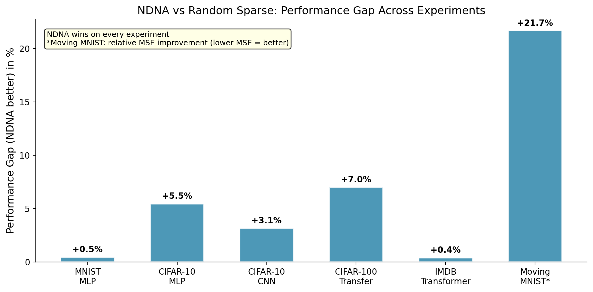
Genome-grown wiring vs random sparse wiring across all experiments. The genome wins everywhere. The biggest gap is on Moving MNIST video (+21.7%), where random wiring completely falls apart but the genome maintains near-dense performance.
Genome vs Dense Networks
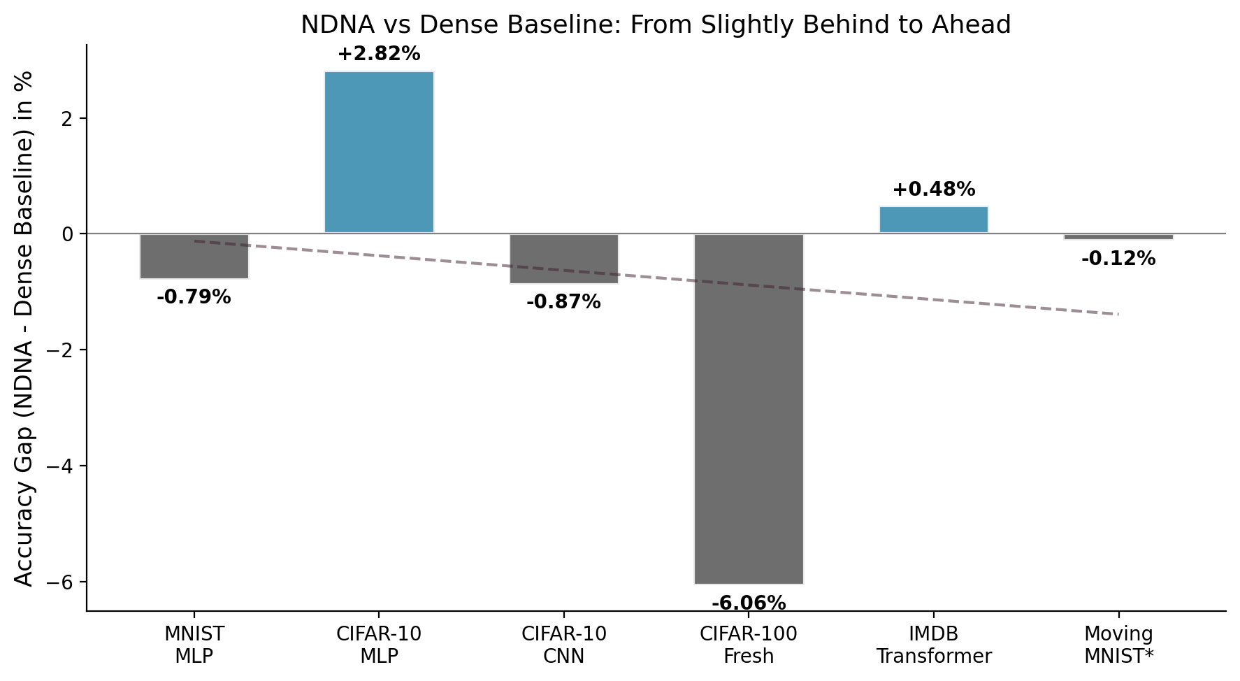
Comparing the genome against fully-connected dense networks. On IMDB sentiment analysis, the genome transformer (85.05%) beats the dense transformer (84.57%) while using only 22.1% of possible connections. Sometimes, less is more, if you pick the right connections.
Cross-Task Transfer
One of the most striking findings. The CIFAR-100 result in the table uses a genome that was trained on CIFAR-10, a different (simpler) dataset. We did not retrain the genome for CIFAR-100. We just took the wiring pattern it learned on CIFAR-10 and used it directly on CIFAR-100, only retraining the network weights.
It still beat random sparse wiring by 7.01 percentage points.
This is significant because it suggests the genome is not just memorizing a wiring pattern for one specific task. It is learning something more general: a reusable principle about how information should flow through a network. Like how the same road network in a city could serve different types of traffic.
Topology Convergence
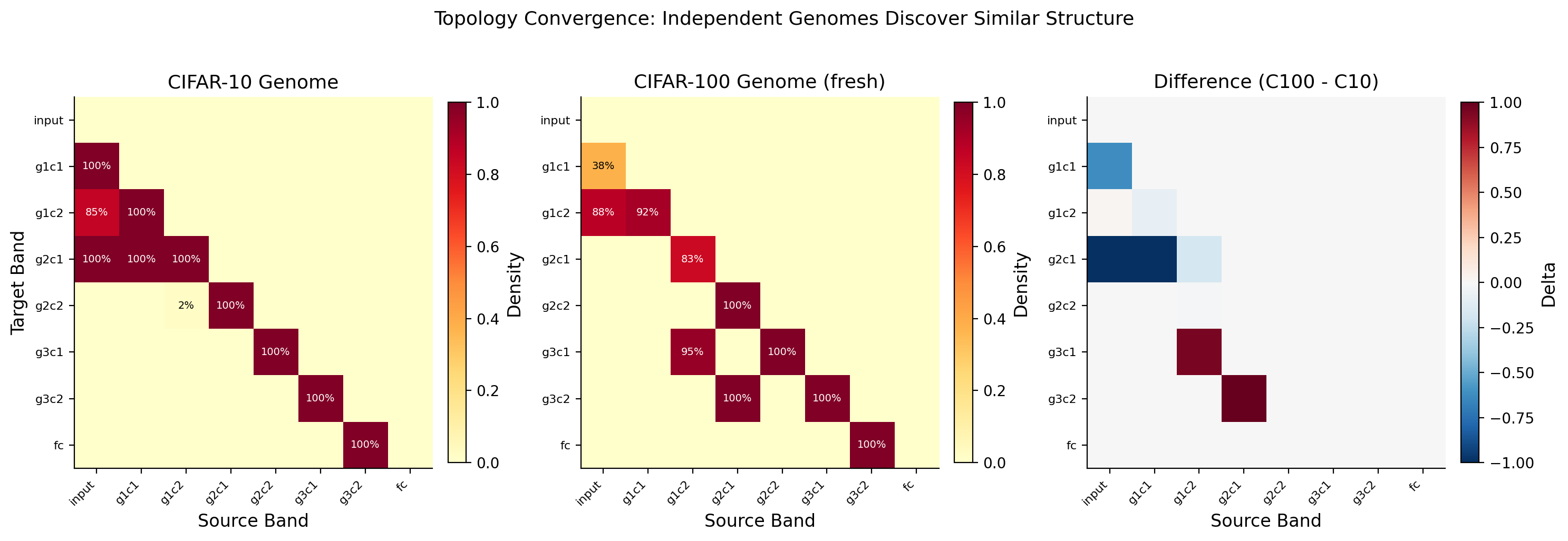
This graph shows how quickly the genome settles on its wiring pattern during training. The structure (which connections exist) stabilizes well before the network weights do. The genome figures out the right architecture early, then the weights spend the rest of training optimizing what they do within that structure. Structure first, then details.
Transformers Too
NDNA is not limited to simple networks. It also works on transformers, the architecture behind models like ChatGPT and other large language models. On IMDB sentiment analysis (classifying movie reviews as positive or negative), the genome-grown transformer beats both the random sparse version and the standard dense version.
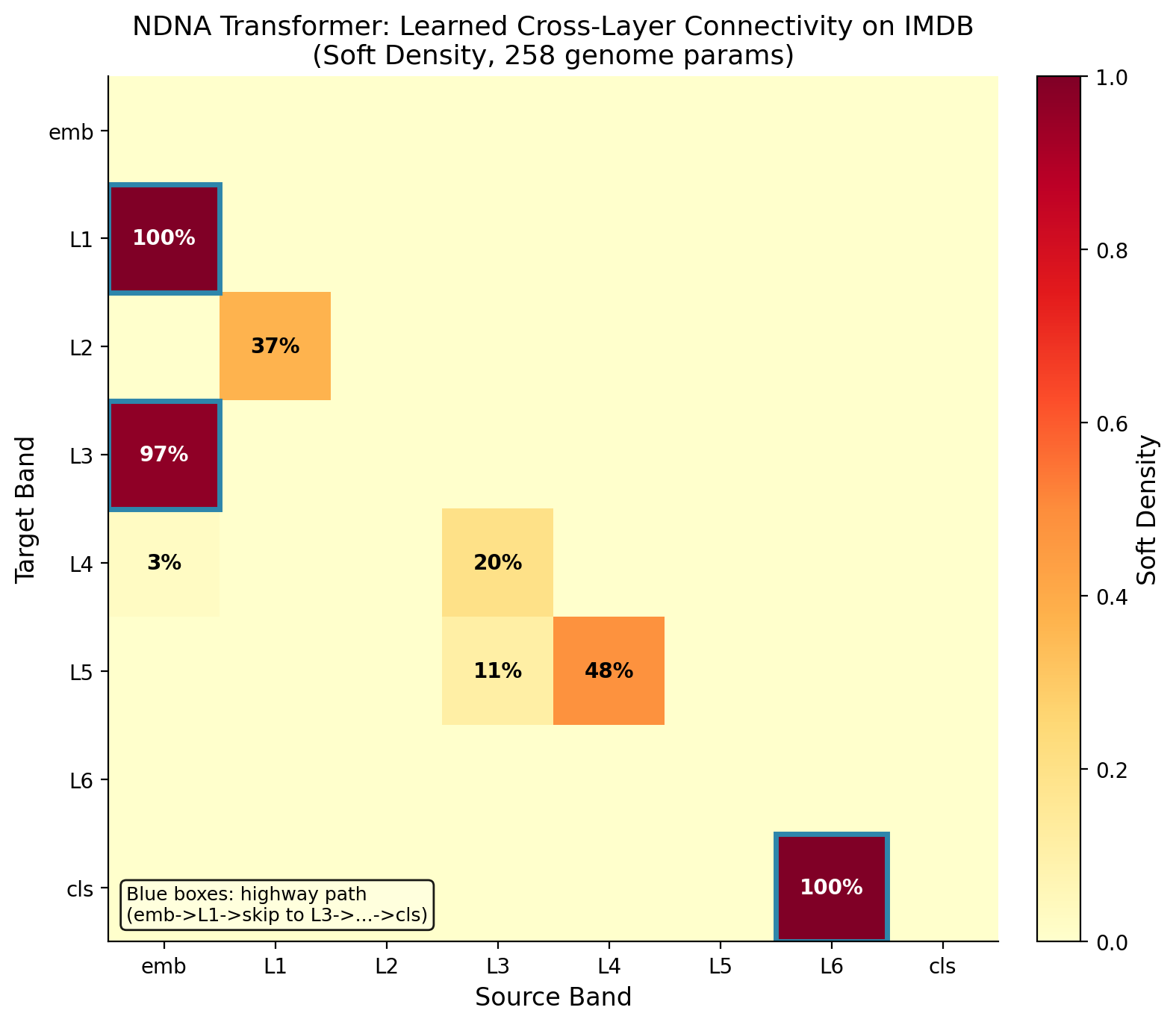
A heatmap showing which connections the genome chose to grow in the transformer. Each cell represents a potential connection between components (attention heads, feed-forward neurons). Bright = connected, dark = disconnected. The genome creates structured patterns, not random noise. It selectively connects the components that work well together.
Video: Where the Gap Gets Huge
The most dramatic result came from video prediction. We trained a video transformer on Moving MNIST (bouncing digit sequences) and asked the genome to learn which frames should attend to which frames, and which spatial patches should attend to which spatial patches.
This required a "factored" genome: instead of one genome controlling everything, we split it into three parts. A temporal genome (74 parameters) that decides which frames connect to which. A spatial genome (74 parameters) that decides which patches within a frame connect to which. And the original depth genome (226 parameters) that controls the feed-forward layers. Total: 374 parameters controlling 307,300 connections.
The genome matched the dense baseline almost exactly (MSE 62.23 vs 62.15). But random sparse wiring at the same density scored 79.44, a 21.7% worse prediction quality. This is by far the largest gap in any of our experiments.
Why is the gap so big? Because video has structure that random wiring cannot capture. The genome learned two things that make intuitive sense:
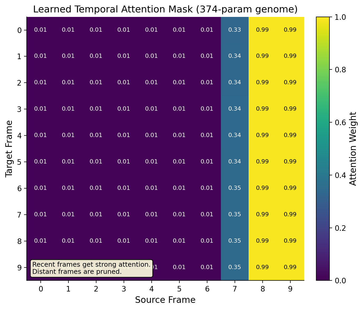
What the temporal genome learned. Recent frames (8 and 9) get strong connections (0.90+). Distant frames (0-6) get almost none (< 0.01). The genome discovered that recent history matters most for prediction, a principle called temporal recency, without being told.
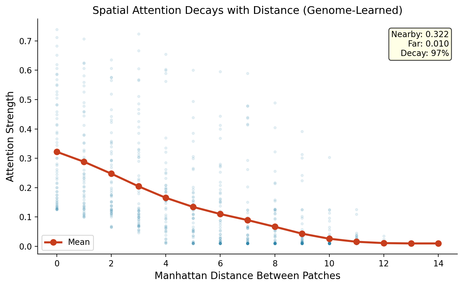
What the spatial genome learned. Nearby patches connect strongly (0.32). Distant patches barely connect (0.01). Attention strength decays 97% with distance. The genome rediscovered spatial locality: pixels near each other matter more to each other than pixels far away.
Random wiring cannot discover these patterns. It connects frames and patches with equal probability, wasting connections on irrelevant relationships. The genome focuses connections where they matter: recent time, nearby space. This is why the gap between genome and random is 21.7% on video, compared to 0.39% to 7.01% on simpler tasks.
The Three Design Principles
Default disconnected. All connections start as off. The genome must actively decide to grow each one. This is the opposite of pruning (start with everything connected, then cut). Growing from nothing is harder, but it means every connection has to prove its worth.
Type-based compatibility. Neurons are assigned "types" based on where they sit in the network. Whether two neurons connect depends on whether their types are compatible, as defined by the genome. This lets a tiny genome express complex wiring patterns across millions of connections without storing each one individually.
Metabolic cost. Growing a connection costs something. A penalty term in training punishes the genome for maintaining too many connections. Just like biological brains conserve energy by keeping only useful synapses, the genome is forced to be selective.
Architecture Support
The genome works across four types of neural network:
- MLP (Multi-Layer Perceptron): The simplest type of neural network. Layers of neurons in sequence. Used for tabular data and basic classification.
- CNN (Convolutional Neural Network): Specialized for images. Uses filters that scan across pixels. The genome controls which filters connect to which.
- Transformer: The architecture behind modern language models. Uses "attention" to relate different parts of the input to each other. The genome controls which attention heads and processing layers connect.
- Video Transformer: Extends the transformer to video by adding temporal attention (across frames) and spatial attention (within frames). The genome controls both dimensions with a factored design: separate temporal and spatial sub-genomes.
Try It
git clone https://github.com/tejassudsfp/ndna.git
cd ndna
pip install -r requirements.txt

# Train genome on MNIST
python3 run.py train

# CIFAR-10 CNN
python3 run.py cnn

# Transfer CIFAR-10 genome to CIFAR-100
python3 run.py transfer100

# Genome transformer on IMDB
python3 run.py transformer

# Video transformer on Moving MNIST
python3 run.py video
Pre-trained genomes are available on Hugging Face.
What Came Next
We scaled NDNA to GPT-2 Small (124M parameters). A 354-parameter genome controls 35.4 million connections at 99,970:1 compression. It beats GPT-2 on 3 benchmarks. Read about it here: Scaling Neural DNA to GPT-2.
Links
- Paper 1: Neural DNA: A Compact Genome for Growing Network Architecture
- Paper 2: Scaling Neural DNA to GPT-2
- Code: GitHub
- Pre-trained Genomes: Hugging Face
- GPT-2 Model: HuggingFace
- Interactive Visualization: ndna.tejassuds.com
Citation
@article{sudarshan2026ndna,
  title={Neural DNA: A Compact Genome for Growing Network Architecture},
  author={Sudarshan, Tejas Parthasarathi},
  year={2026},
  doi={10.5281/zenodo.19248389}
}