Scaling Neural DNA to GPT-2
354 parameters wire a language model. 99,970:1 compression. Beats GPT-2 on 3 benchmarks.
Quick Recap
If you have not read the first NDNA post, here is the one-paragraph version:
NDNA is a tiny "genome" (fewer than 400 numbers) that learns which connections in a neural network should exist and which should not. Instead of starting with every neuron connected to every other neuron (the standard approach), the genome grows connections selectively, like how biological brains wire themselves during development. In the first paper, we tested this on small networks (MNIST, CIFAR-10, IMDB sentiment, video prediction) and showed that genome-grown wiring consistently beats random wiring and sometimes even beats fully-connected networks.
The question was: does this scale?
The Experiment
GPT-2 Small is a language model built by OpenAI in 2019. It has 124 million parameters, 12 layers, and was trained to predict the next word in a sentence. It is not the largest model by today's standards, but it is a real production-scale transformer. The kind of model that actually works on real text.
We took GPT-2 Small and gave a genome control over two specific parts of each layer:
-
The attention output projection (W_O): After the attention mechanism figures out which words to pay attention to, this layer combines those attention results into a single output. It is a 768x768 matrix in each layer.
-
The feed-forward first layer (FF1): Each transformer layer has a two-layer feed-forward network. The first layer expands the representation from 768 dimensions to 3072 dimensions. It is a 3072x768 matrix in each layer.
Combined, that is 2.95 million connections per layer. Across 12 layers: 35.4 million connections controlled by a genome of 354 parameters.
That is a 99,970:1 compression ratio. One genome parameter for every 100,000 connections.
Everything else (the query, key, value projections that drive attention, the second feed-forward layer, all the layer normalization, the residual connections, and the language model head) trains normally without any genome control.
What Happened
We trained the genome and the model weights together from scratch on OpenWebText (the same dataset used for the original GPT-2). Single A100 GPU. 52,700 iterations. 25.9 billion tokens.
Then we evaluated on nine standard benchmarks and compared against GPT-2's published numbers.
| Benchmark | NDNA GPT-2 | GPT-2 Small | Result |
|---|---|---|---|
| WikiText-103 PPL | 36.0 | 37.5 | Beats GPT-2 |
| Penn Treebank PPL | 59.4 | 65.9 | Beats GPT-2 |
| LAMBADA PPL | 22.2 | 35.1 | Beats GPT-2 |
| LAMBADA ACC | 30.8% | 46.0% | 67% of GPT-2 |
| HellaSwag ACC | 28.7% | 31.2% | 92% of GPT-2 |
| CBT-CN ACC | 82.7% | 87.7% | 94% of GPT-2 |
| CBT-NE ACC | 74.5% | 83.4% | 89% of GPT-2 |
The model beats GPT-2 on all three perplexity benchmarks. WikiText-103 by 4%, Penn Treebank by 10%, LAMBADA by 37%.
On accuracy benchmarks (where the model has to pick the single correct answer), it reaches 89-94% of GPT-2's performance. The gap is real, but the model was also trained on roughly half the compute GPT-2 used.
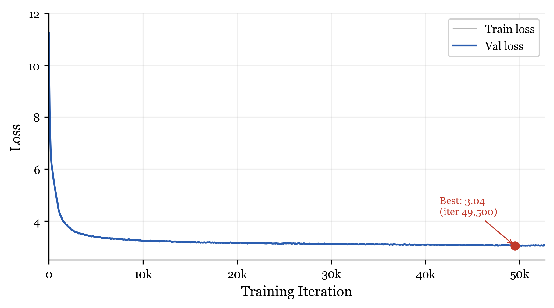
Validation loss over training. The NDNA model reaches 3.04 at iteration 49,500.
Perplexity vs Accuracy: Why Both Matter
Quick detour, because this confused me at first too.
Perplexity measures how well the model understands language overall. Lower is better. If a sentence says "The cat sat on the ___", perplexity measures whether the model puts high probability on reasonable next words ("mat", "couch", "floor") and low probability on unreasonable ones ("algebra", "helicopter").
Accuracy measures whether the model picks the single right answer. If the answer is "mat", accuracy only cares if "mat" was the model's top prediction.
Our model beats GPT-2 on perplexity: it builds a better understanding of which words are likely in context. But it trails on accuracy: it is less confident about picking one single answer.
Think of it this way. If you asked two students to predict what comes next in a story, one student (GPT-2) is very decisive but sometimes guesses wrong. The other student (NDNA) has a better overall understanding of the story but hedges more on their final answer. Perplexity rewards the one who understands better. Accuracy rewards the one who commits harder.
With one-third of its connections permanently disabled, the NDNA model has fewer pathways for sharpening its predictions to a single answer. But the connections it does have are the right ones, so its overall understanding is actually better.
The Topology
This is where it gets interesting.
The genome does not just randomly prune some connections. It discovers a clear pattern:
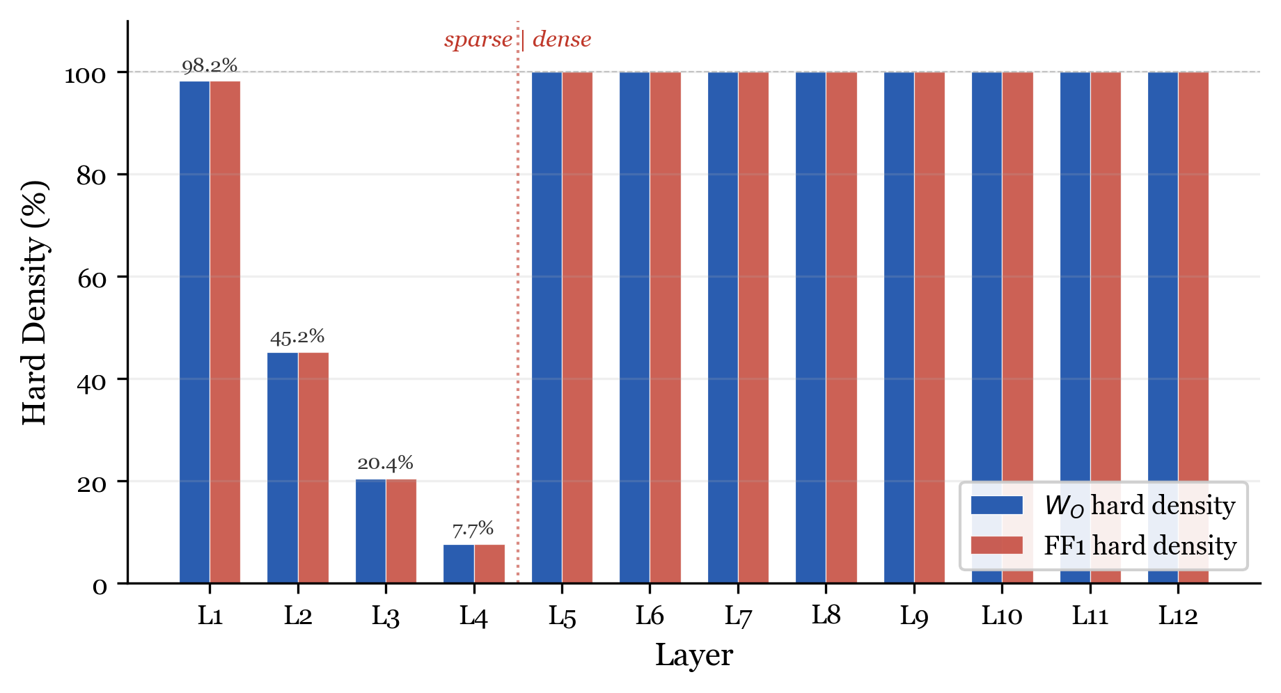
Final per-layer density. The genome creates two distinct zones: sparse (layers 1-4) and dense (layers 5-12).
| Layer | 1 | 2 | 3 | 4 | 5 | 6 | 7 | 8 | 9 | 10 | 11 | 12 |
|---|---|---|---|---|---|---|---|---|---|---|---|---|
| Density | 98.2% | 45.2% | 20.4% | 7.7% | 100% | 100% | 100% | 100% | 100% | 100% | 100% | 100% |
Layers 5 through 12 are fully connected. Every single connection survives. The genome decided these layers need all their wiring.
Layers 1 through 4 are progressively pruned in a strict gradient: 98%, 45%, 20%, 8%. Layer 4 loses 92% of its connections.
Overall: one-third of all masked connections are permanently off. The model operates with 23.6 million active connections out of 35.4 million possible.
Nobody told the genome to do this. It discovered on its own that deep layers are indispensable and shallow layers are largely redundant. This is consistent with findings in the pruning literature, where researchers have observed that some layers in transformers tolerate significantly more sparsity than others. The genome rediscovered this from scratch.
Within each layer, the attention output (W_O) and feed-forward (FF1) masks have nearly identical density. The genome treats each layer as a unit: if a layer is important, both its attention output and feed-forward computation get full wiring. If a layer is expendable, both get pruned equally. This same pattern appeared in the small-scale IMDB transformer experiment from Paper 1.
The Four Phases
The genome does not just settle on a topology immediately. It goes through four distinct phases during training, and watching this process is genuinely fascinating. You can see this play out in real time on the interactive visualization.
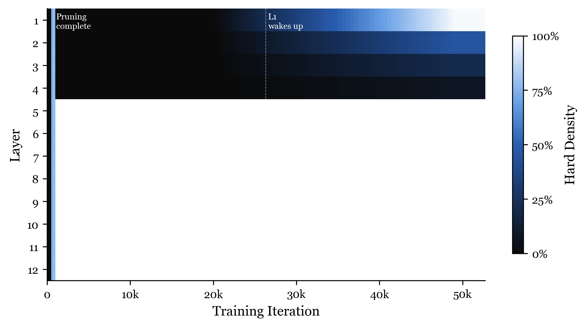
Per-layer density over training. Each row is a layer (1-12). Bright = connected, dark = disconnected. The four phases are clearly visible.
Phase 1: Over-activation (iterations 0 to 200)
The genome starts by turning almost everything on. Within the first 200 iterations, 83% of all connections are active. The genome has not yet learned what to prune. It is hedging its bets.
This is like a new employee on their first week who tries to attend every meeting and respond to every email. They do not know what matters yet, so they treat everything as important.
Phase 2: Aggressive pruning (iterations 200 to 800)
By iteration 800, the genome makes a dramatic decision: it prunes layers 1 through 4 to 0% hard density. Zero. Not a single connection active in those layers.
The model is now running with only 8 of its 12 layers doing any real work through the masked projections. The other 4 layers still exist (their residual connections and layer normalization still function), but their attention output and feed-forward computations contribute nothing.
This is like that same employee, a few months in, realizing they only need to be in 8 of those 12 meetings. They drop the others completely.
Phase 3: Stable learning (iterations 800 to 25,000)
The topology locks in. The genome holds steady. The model spends the next 24,200 iterations learning language within this fixed sparse structure. Validation loss drops from 7.99 to 3.18 during this phase.
This is the longest and most productive phase. The structure is set. Now the network just learns.
Phase 4: Layer 1 resurrection (iterations 25,000 to 50,000)
This is the most unexpected finding.
After being completely disconnected for 25,000 iterations, layer 1 starts coming back to life. Its density rises from 0% and eventually reaches 98.2%. The genome changed its mind.
Layers 2, 3, and 4 stay pruned. Only layer 1 gets reconnected.
What happened? Our hypothesis: in the early phases, the model learned basic language using layers 5-12. The residual stream carried information through the dead layers just fine. But as the model approached its quality ceiling, it discovered that layer 1's attention output projection provides useful low-level features (token-level patterns, basic syntax) that improve perplexity. So the genome reconnects it.
This is reminiscent of biological development, where genes activate, deactivate, and reactivate at different developmental stages. The genome does not lock in its decisions permanently. It stays plastic and revises its structural hypothesis as training progresses, right up until the temperature reaches its maximum and the topology crystallizes.
You can scrub through this entire process on the interactive visualization. Move the timeline slider and watch layers light up, go dark, and come back to life.
Layer-by-Layer Breakdown
Here is what the genome decided for each of GPT-2's 12 layers. The bar width represents how many connections survived.
The sharp boundary between layer 4 (7.7%) and layer 5 (100%) is the most striking feature. The genome splits the network into two zones with almost no transition.
Key Moments During Training
Explore the full training timeline at ndna.tejassuds.com, where you can scrub through every iteration and watch these events happen in real time.
Compression at Scale
The compression ratio keeps getting better as the network gets bigger:
| Experiment | Genome Params | Connections | Compression |
|---|---|---|---|
| MNIST MLP | 226 | 174K | 770:1 |
| CIFAR-10 MLP | 226 | 1.7M | 7,553:1 |
| IMDB Transformer | 258 | 2.2M | 8,384:1 |
| GPT-2 Small | 354 | 35.4M | 99,970:1 |
The genome grew by 37% (from 258 to 354 parameters) while the connections it controls grew by 16x. Compression scales super-linearly with network size.
This is not an accident. The genome does not store one bit per connection. It stores a developmental program (cell type assignments, compatibility rules) that generates masks for any number of connections through matrix operations. Bigger networks have more connections but the same number of type interactions. So the ratio keeps improving.
If you applied the same genome architecture to GPT-2 XL (1.5 billion parameters), the genome might still be under 500 parameters while controlling hundreds of millions of connections.
What This Means
For AI efficiency
One-third of the connections in layers 1-4 are dead weight. If the genome can figure out which ones to cut, targeted width reduction or layer removal at those positions could produce genuinely smaller, faster models. Not through post-training compression, but by never creating the unnecessary connections in the first place.
For understanding transformers
The genome's topology is a map of what matters in GPT-2. Deep layers need everything. Shallow layers are mostly redundant. Layer 4 can lose 92% of its connections without the model getting worse than GPT-2. That is a strong signal about where the real computation happens in a transformer.
For the genome approach
In Paper 1, we showed NDNA works on toy tasks. The open question was whether it would survive contact with a real model. It did. Same six parameter groups, same type-based compatibility rules, same temperature annealing, same metabolic cost pressure. No modifications. The genome architecture is general enough to scale from MNIST to GPT-2.
Limitations
Being honest about what we did not do:
-
No random sparse baseline. In Paper 1, we compared genome wiring against random sparse wiring at the same density. We did not do this for GPT-2. Training GPT-2 with random 66.7% sparse masks would isolate whether the genome's specific wiring pattern matters, or if any sparse pattern would work.
-
Incomplete training. We trained for 52,700 iterations out of a planned 100,000. The accuracy gap might narrow with more training.
-
Single seed. All results from one random seed (42). More seeds would give confidence intervals.
-
Partial masking. The genome controls 28.4% of the model. Extending it to Q, K, V projections and FF2 would be a more complete test.
What is Next
Random sparse comparison. The most immediate next experiment. Does genome wiring specifically matter, or would any sparse wiring do at this scale?
Larger models. GPT-2 Medium (345M), Large (774M), XL (1.5B). Does the compression ratio keep improving?
Full training. Complete the planned 100,000 iterations to see if the accuracy gap closes.
Broader masking. Give the genome control over Q, K, V projections and the second feed-forward layer. That would increase genome-controlled parameters from 28.4% to over 90%.
Try It
git clone https://github.com/tejassudsfp/ndna.git
cd ndna
pip install -r requirements.txt

# Train GPT-2 Small with NDNA genome (requires A100)
python3 experiments/rung5_gpt2.py

# Evaluate on benchmarks
python3 experiments/eval_full_benchmark.py
Or load the pre-trained model directly:
import torch
from genome.model import Genome, GrownGPT2

ckpt = torch.load("genome_ckpt.pt", map_location="cpu")
genome = Genome(n_types=8, type_dim=8, n_bands=14)
model = GrownGPT2(genome)

model_state = {k.replace("_orig_mod.", ""): v for k, v in ckpt["model"].items()}
genome_state = {k.replace("_orig_mod.", ""): v for k, v in ckpt["genome"].items()}
genome.load_state_dict(genome_state)
model.load_state_dict(model_state, strict=False)

model.hard_masks = True
model.eval()
The pre-trained model and checkpoint are on HuggingFace.
Links
- Paper 1: Neural DNA: A Compact Genome for Growing Network Architecture (small-scale experiments)
- Paper 2: Scaling Neural DNA to GPT-2 (this work)
- Code: GitHub
- Model: HuggingFace
- Interactive Visualization: ndna.tejassuds.com
Citation
@article{sudarshan2026ndna_gpt2,
  title={Scaling Neural DNA to GPT-2: 354 Parameters Wire a Language Model},
  author={Sudarshan, Tejas Parthasarathi},
  year={2026},
  doi={10.5281/zenodo.19390927}
}